How to get around the two issues that speed of computer and the efficiency of the Python implementation on that computer?

Instead of measuring time in milliseconds, we measure time in terms of the number of basic steps executed by the program. It is a more abstract way to think about the measure of time.

For simplicity, we will use a random access machine as our model of computation. In a random access machine, steps are executed sequentially, one at a time. A step is an operation that takes a fixed amount of time, such as binding a variable to an object, making a comparison, executing an arithmetic operation, or accessing an object in memory.

How to deal with the question that program running time measurement depends on the value of input?

We deal with that by moving away from expressing time complexity as a single number and instead relating it to the sizes of the inputs. This allows us to compare the efficiency of two algorithms by talking about how the running time of each grows with respect to the sizes of the inputs.

How about the actual running time of an algorithm depends not only upon the sizes of the inputs but also upon their values?

def linearSearch(L, x): 
    for e in L:
        if e == x: 
            return True
    return False

In general, there are three broad cases to think about:

1. The best-case running time is the minimum running time over all the possible inputs of a given size.For linearSearch, usually it is independent of the size of L.

2. The worst-case running time is the maximum running time over all the possible inputs of a given size. For linearSearch, the worst-case running time is linear in the size of L.

3. By analogy with the definitions of the best-case and worst-case running time,

   the average-case (also called expected-case) running time is the average run- ning time over all possible inputs of a given size. Alternatively, if one has some a priori information about the distribution of input values (e.g., that 90% of the time x is in L), one can take that into account.

Why people usually focus on the worst case?

All engineers share a common article of faith, Murphy’s Law: If something can go wrong, it will go wrong. The worst-case provides an upper bound on the running time. This is critical in situations where there is a time constraint on how long a computation can take.

Why do we use asymptotic notation as a formal way to talk about the relationship between the running time of an algorithm and the size of its inputs?

The underlying motivation is that almost any algorithm is sufficiently efficient when run on small inputs. What we typically need to worry about is the efficiency of the algorithm when run on very large inputs. As a proxy for “very large,” asymptotic notation describes the complexity of an algorithm as the size of its inputs approaches infinity.

What is the most commonly used asymptotic notation?

“Big O” notation is used to give an upper bound on the asymptotic¹ growth (often called the order of growth) of a function. For example, the formula f(x) ∈ O(x²) means that the function f grows no faster than the quadratic polynomial x², in an asymptotic sense.

What do we mean saying “the complexity of f(x) is O(x²)”?

The difference between a function being “in O(x²)” and “being O(x²)” is subtle but important. Saying that f(x) ∈ O(x²) does not preclude the worst-case running time of f from being considerably less than O(x²).

When we say that f(x) is O(x²), we are implying that x² is both an upper and a lower bound on the asymptotic worst-case running time. This is called a tight bound.

Some of the most common instances of Big O

In each case, n is a measure of the size of the inputs to the function.

• O(1) denotes constant running time.
• O(log n) denotes logarithmic running time.
• O(n) denotes linear running time.
• O(n log n) denotes log-linear running time.
• O(n^k) denotes polynomial running time. Notice that k is a constant.
• O(cⁿ) denotes exponential running time. Here a constant is being raised to a power based on the size of the input.

Example codes for logarithmic complexity

def intToStr (i):
   """ 假设 i 是非负整数
      返回一个表示 i 的十进制字符串
      """
   digits = '0123456789'
   if i == 0:
      return '0'
   result = ''
   while i > 0:
      result = digits [i%10] + result
      i = i//10
   return result

The complexity of intToStr is O(log(i)).

def addDigits(n):
    """ Assumes n is a nonnegative int
        Returns the sum of the digits in n""" 
    stringRep = intToStr(n)
    val = 0
    for c in stringRep:
        val += int(c)
    return val

It runs in time proportional to O(log(n)) + O(log(n)), which makes it O(log(n)).

Example codes for linear complexity

def addDigits(s):
    """ Assumes s is a str each character of which is a
        decimal digit.
        Returns an int that is the sum of the digits in s"""
    val = 0
    for c in s:
        val += int(c) 
    return val

It is linear in the length of s, i.e., O(len(s)).

def factorial(x):
    """ Assumes that x is a positive int
        Returns x!""" 
    if x == 1:
       return 1
    else:
        return x*factorial(x-1)

There are no loops in this code, so in order to analyze the complexity we need to figure out how many recursive calls get made.

Example codes for log-linear complexity

Many practical algorithms are log-linear. The most commonly used log-linear algorithm is probably merge sort, which is O(n log(n)), where n is the length of the list being sorted.

Example codes for polynomial complexity

def isSubset (L1, L2):     # O (len (L1))*O (len (L2))
   """ Assumes L1 and L2 are lists.
       Returns True if each element in L1 is also in L2
       and False otherwise. """
   for e1 in L1:           # O (len (L1))
      matched = False
      for e2 in L2:        # O (len (L2))
         if e1 == e2:
            matched = True
            break
      if not matched:
         return False
   return True

def intersect (L1, L2):
   """ Assumes: L1 and L2 are lists
      Returns a list without duplicates that is the intersection of
      L1 and L2 """
   # Build a list containing common elements
   tmp = []
   for e1 in L1:         # O (len (L1))
      for e2 in L2:      # O (len (L2))
         if e1 == e2:
            tmp.append (e1)
            break
   # Build a list without duplicates
   result = []
   for e in tmp:        # O (len (tmp))
      if e not in result:   # O (len (result))
         result.append (e)
   return result

Example codes for exponential complexity

def getBinaryRep (n, numDigits): # O (log2 (n))
   """ Assumes n and numDigits are non-negative ints
       Returns a str of length numDigits that is a binary
       representation of n """
   result = ''
   while n > 0:
      result = str (n%2) + result
      n = n//2
   if len (result) > numDigits:
      raise ValueError ('not enough digits')
   for i in range (numDigits - len (result)):
      result = '0' + result
   return result

def genPowerset (L): # O (2**len (L))*O (len (L))
   """ Assumes L is a list
       Returns a list of lists that contains all possible
       combinations of the elements of L. E.g., if
       L is [1, 2] it will return a list with elements 
       [], [1], [2], and [1,2]."""
   powerset = []
   for i in range (0, 2**len (L)): # O (2**len (L)) 区分先后的组合
      binStr = getBinaryRep (i, len (L))
      subset = []
      for j in range (len (L)): # O (len (L))
         if binStr [j] == '1':
            subset.append (L [j])
      powerset.append (subset)
   return powerset

The algorithm is a bit subtle. Consider a list of n elements. We can represent any combination of elements by a string of n 0’s and 1’s, where a 1 represents the presence of an element and a 0 its absence. The combination containing no items is represented by a string of all 0’s, the combination containing all of the items is represented by a string of all 1’s, the combination containing only the first and last elements is represented by 100…001, etc.

Generating all sublists of a list L of length n can be done as follows:

• Generate all n-bit binary numbers. These are the numbers from 0 to 2 .
• For each of these 2ⁿ +1 binary numbers, b, generate a list by selecting those n elements of L that have an index corresponding to a 1 in b. For example, if L is [‘x’, ‘y’] and b is 01, generate the list [‘y’].

Comparisons of Complexity Classes

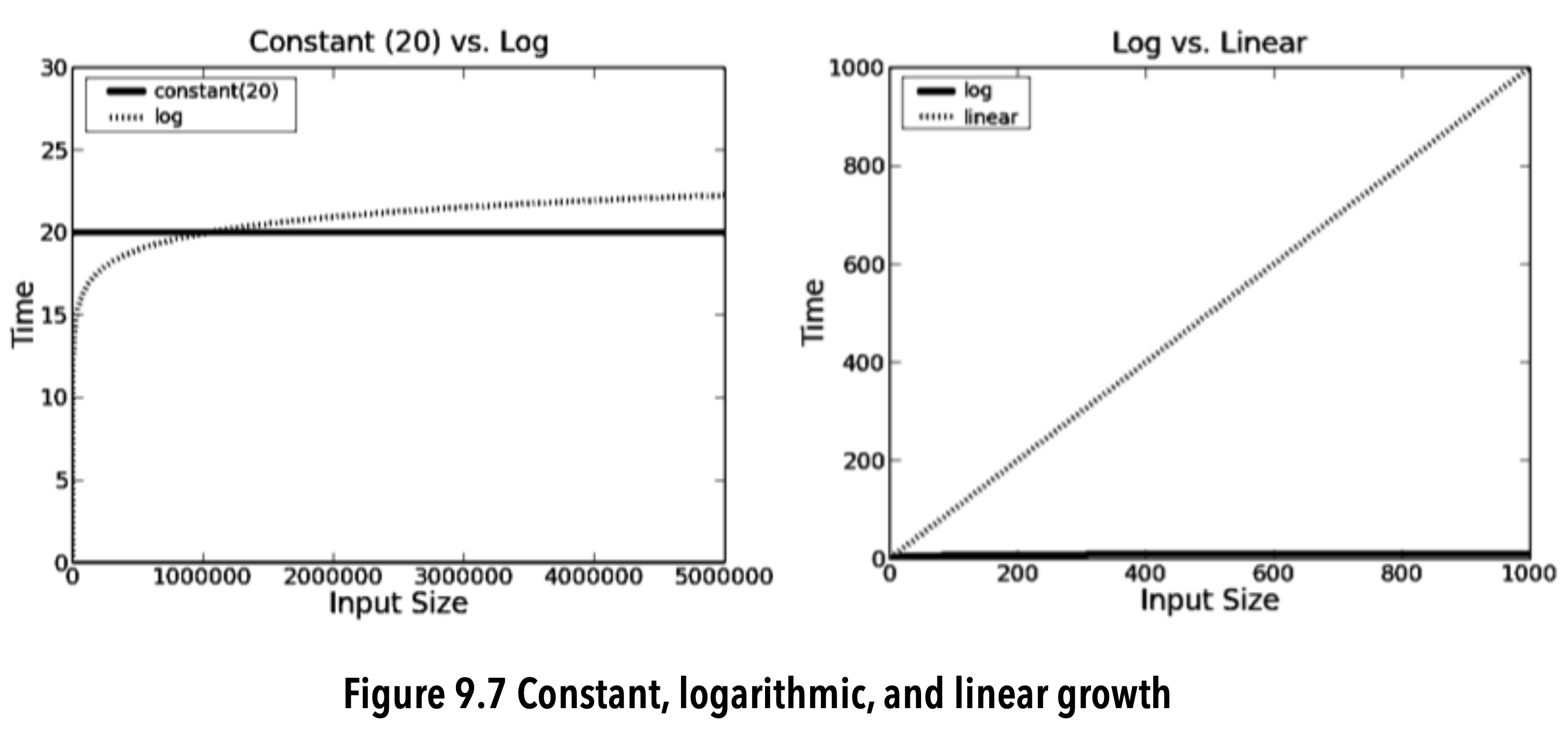
image-20200609203905121

• Logarithmic algorithms are almost as good as constant-time ones.
• Most of the time a linear algorithm is acceptably efficient.

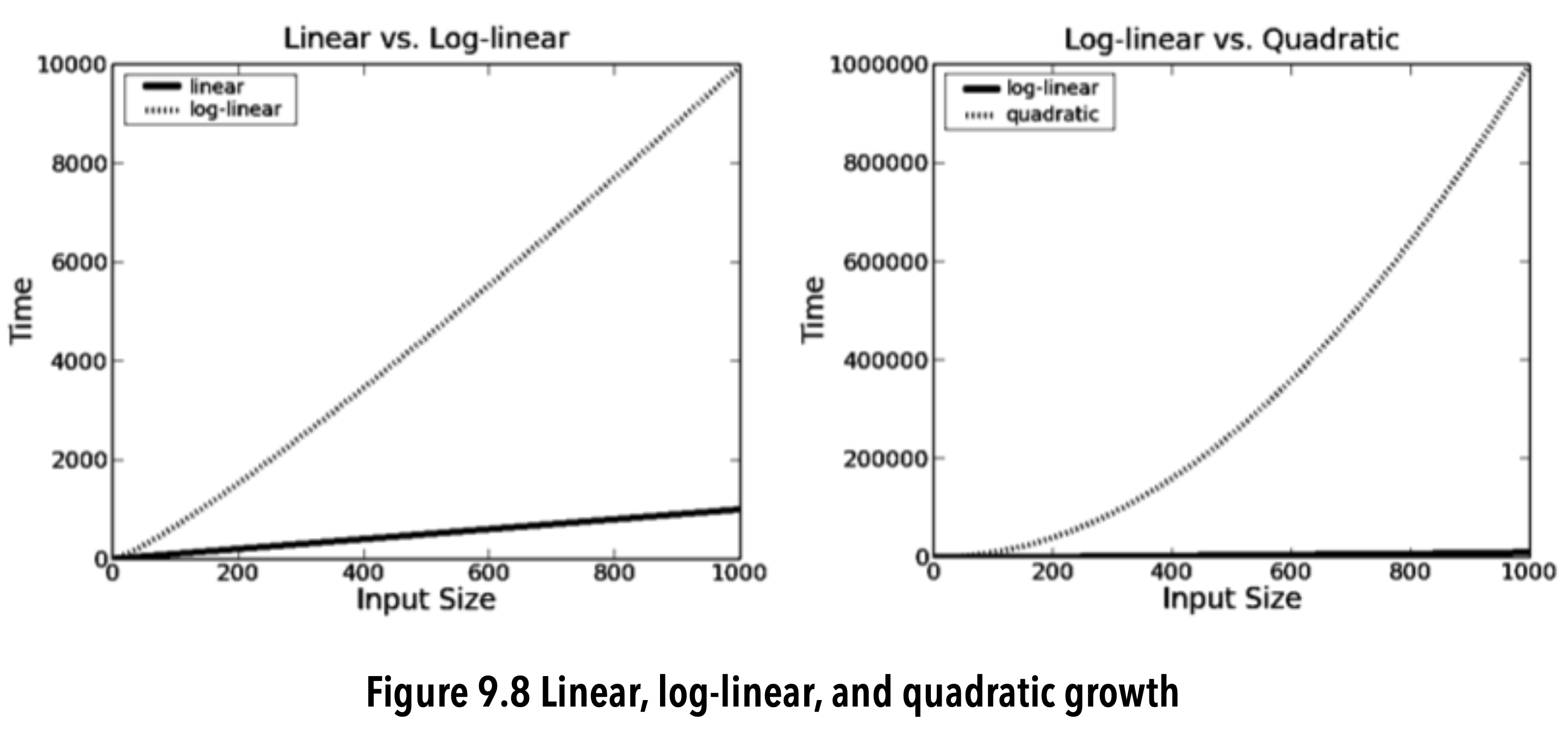
image-20200609203927517

• In many practical situations, O(n log(n)) is fast enough to be useful.
• There are many situations in which a quadratic rate of growth is prohibitive.

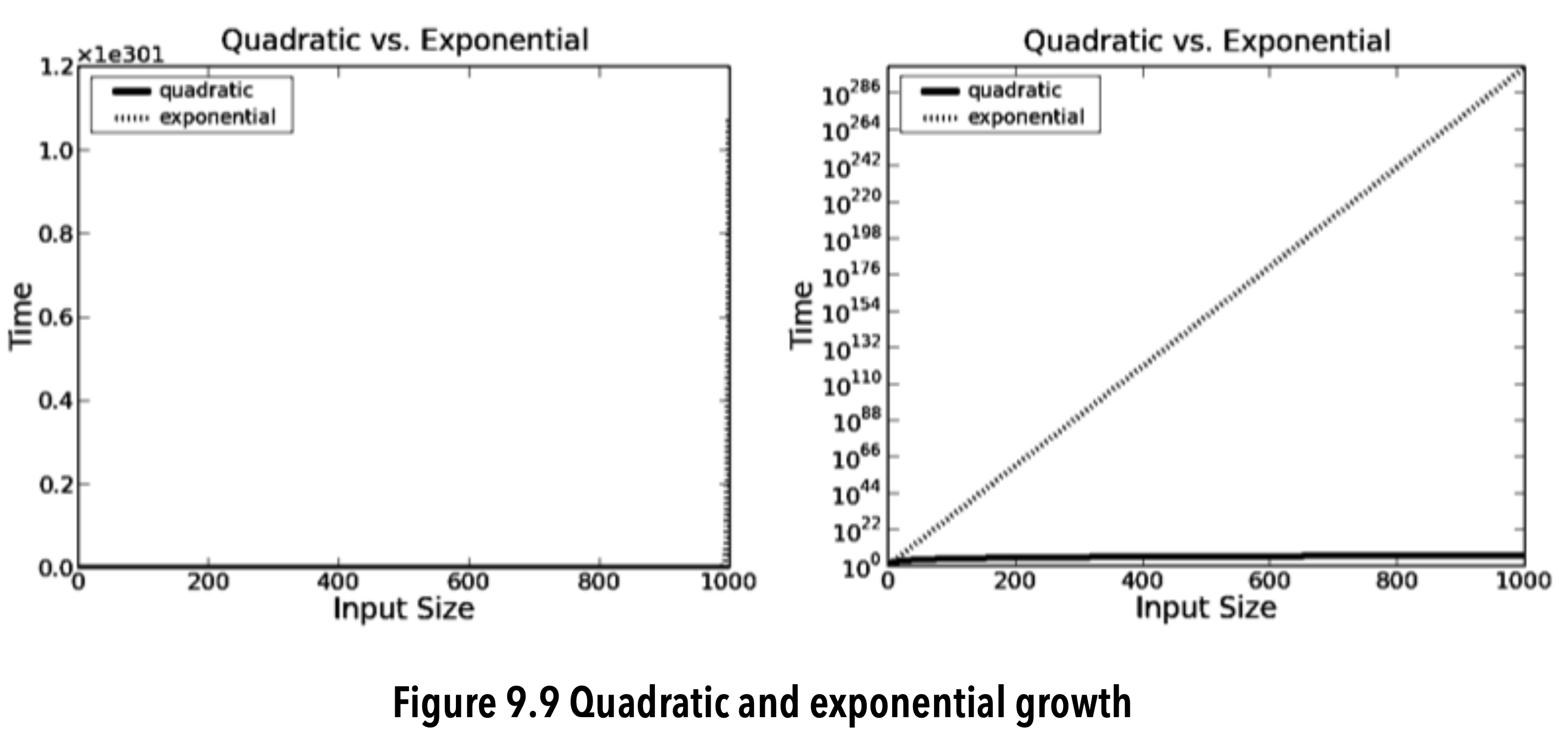
image-20200609203956520

• The notation x1e301 on the top left means that each tick on the y-axis should be multiplied by 10³⁰¹.
• Exponential algorithms are impractical for all but the smallest of inputs.

2020-06-09